
Synergetic Lattice Field Theory
CONTENTS
SYNERGETIC LATTICE FIELD THEORY & ELEMENTARY PARTICLES
Electrons in the Synergetic Field
Synergetic lattice field theory (SLFT) lays out a well-defined set of localized deformations of the synergetic field. It identifies these local deformations with the standard model’s elementary fermions. As illustrated below, SLFT identifies electrons with local octahedral contractions of the field’s isomorphic vector equilibria. The localized contractions that define elementary particles, such as electrons, are seamlessly embedded within the synergetic field, and they gradually merge into a surrounding ocean of the synergetic field in its isomorphic configuration.

Figure 1: Electrons in the Synergetic Field. A local, two-dimensional cross-section through the synergetic field in a region of local, octahedral contraction associated with an electron. This figure shows the very central area of an electron deformation of the synergetic field. This figure shows a gradual rate of change in contractions between neighboring vector equilibria, but it is still a much greater rate of change in contractions than is expected to exist in nature. The illustration shows only the left-handed, octahedrally contracted set of vector equilibria. The complementary right-handed, cuboctahedrally expanded vector equilibria are omitted for visual clarity.
Motion of Electrons through the Synergetic Field
The illustration above shows the center portion of an electron at a fixed position within the synergetic field. However, electrons are never actually stationary in the field. The illustration below provides a picture of a moving electron represented as a soliton-like wave of contraction moving through the synergetic field. The motion of the electron through the synergetic field is nothing other than the motion of such an octahedral “wave pulse”. The individual components of the underlying field, its constituent vector equilibria, are not themselves moving from one place to another in the field. Instead, a well-defined and stable pattern of localized contraction, formed within, and from, the synergetic field, itself, is moving through the field.
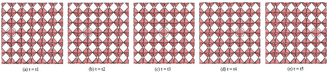
Figure 2: Electron Motion Through the Synergetic Field. The motion of an octahedral wave pulse (i.e. electron) through a local slice of the synergetic field. The circles in these figures highlight which vector equilibrium in each of the five sequential “snap shots” of the synergetic field is contracted completely to its octahedral phase. Electron motion animation: Animation.
Borrowing from Einstein and Infeld [1] one can think of these wave pulses, which SLFT uses to define elementary particles, as moving areas of local “field intensities”. Fuller would likely have referred to these wave pulses as the motion of “pattern integrities” [2].
Neutrinos in the Synergetic Field
In a similar manner, SLFT identifies neutrinos with localized, icosahedral contractions of the synergetic field’s isomorphic vector equilibria.

Figure 3: Neutrinos in the Synergetic Field. The pattern of contraction in the synergetic field that is associated with the formation of a neutrino is visually subtle when compared with the pattern of contraction associated with an electron. The localized, icosahedral contraction of the synergetic field shown in the illustration represents only a modest contraction of the field relative to its uncontracted, isomorphic state. The centermost vector equilibrium in the illustration is in its icosahedral configuration while the vector equilibria around the edges of the figure are in their isomorphic configurations. This can be visually discerned if one looks very closely and carefully at the illustration’s centermost vector equilibrium compared to its perimeter vector equilibria. (Animation.)
Quarks in the Synergetic Field
SLFT identifies quarks with local tetrahedral contractions of the field’s isomorphic vector equilibria.

Figure 4: Tetrahedral Jitterbug Transformation. The sequential contraction of the vector equilibrium from its cuboctahedral phase (far left) to its tetrahedral phase (far right). Fuller also discovered this variant of the vector equilibrium’s jitterbug transformation [3]. During this contraction two oppositely oriented square openings in the vector equilibrium progressively pinch together in orthogonal directions until the tetrahedral phase is reached. In this instance the two square openings that pinch together are the left and right facing openings. The left opening pinches together parallel to the page’s vertical axis. The right opening pinches together parallel to an axis that runs in-and-out of the page. (Animation.)
Just as the electron-octahedral and neutrino-icosahedral contractions can be embedded within the synergetic field, so can the quark-tetrahedral contraction. Because of the higher geometric complexity of this contraction, especially when embedded within the field, it is a little harder to visualize. A very small section of the synergetic field illustrating this contraction at the very center of a quark is shown below. As with the electron and neutrino deformations, this center most deformation associated with a quark gradually merges into a surrounding ocean of isomorphic vector equilibria. The manner in which the vector equilibrium's tetrahedral contraction can be embedded within the isotropic vector matrix, as a whole, was an important discovery of SLFT—it is key to SLFT's ability to model quarks.

Figure 5: Quarks in the Synergetic Field. The local deformation of the synergetic field associated with quarks starts where the local electron-octahedral contraction leaves off (see Figure 7, below). Figure (a) shows the local deformation as it would appear at the center of an electron for a very small array of four vector equilibria in their octahedral phases, and nine surrounding vector equilibria underneath them, in their cuboctahedral phases. The sequential transformation of this array of vector equilibria from an “electron” configuration to a “quark” configuration is illustrated in figures (b) through (f). The nine cuboctahedral phase vector equilibria transform to their tetrahedral phases while the octahedral phase vector equilibria rotate around their vertex axes. Figure (f) shows the configuration of the synergetic field at the very center of a local field deformation associated with a quark. (Animation.) A separate animation shows the motion of a quark through a two-dimensional slice of the synergetic field: Animation.
Quark Colors, Flavors, and Fractional Electric Charges
It turns out that the vector equilibrium's tetrahedral contraction, as shown in Figure 5 above, can occur in six symmetrical orientations when embedded within the synergetic field. SLFT maps these six symmetrically differentiated contractions of the vector equilibrium to the six permutations of quark color and flavor described by the standard model. In addition, certain internal geometric transformations of the vector equilibrium that occur when it undergoes its tetrahedral contraction provide geometric explanations for the 1/3 and 2/3 fractional electrical charges carried by quarks. Full discussions and explanations of these mappings between quark colors, flavors, and fractional electric charges, and the geometry of the synergetic field are provided in the full paper on SLFT.
Negative Mass in the Synergetic Field
The geometry of the synergetic field, itself, naturally gives rise to negative-mass particles. This is a result of the synergetic field’s construction from equal numbers of left-handed and right-handed isomorphic vector equilibria, which each respectively contract in either a left-handed or a right-handed manner.

Figure 6: Left-Handed & Right-Handed Jitterbug Transformations. The upper row in the figure shows a vector equilibrium contracting from its cuboctahedral phase (far left) to its octahedral phase (far right), in a “left-handed” sense. The lower row similarly shows a vector equilibrium contracting from its cuboctahedral phase to its octahedral phase in a “right-handed” sense. The upper right triangle in a vector equilibrium is arbitrarily selected as a reference point for determining the handedness of the vector equilibrium’s contraction. In the upper row, this triangle is rotating in left-handed, clockwise sense as the vector equilibrium’s contraction progresses from left to right. In the lower row, this triangle is rotating in right-handed, counterclockwise sense as the vector equilibrium’s contraction progresses from left to right. As the left-handed and right-handed vector equilibriums progressively contract from their cuboctahedral phases to their octahedral phases, all of their corresponding triangles rotate in opposite directions. (Animation.)
These left-handed and right-handed contractions can occur to vector equilibria embedded within the synergetic field. The left-handed and right-handed contractions respectively cause associated left-handed or right-handed twisting (torsion) within the field. The resulting positive and negative torsion in the field gives rise respectively to positive-mass or negative-mass particles.

Figure 7: Positive and Negative Mass in the Synergetic Field. Two identical clusters of 16 isomorphic phase vector equilibria are shown at the top positions in this figure’s left and right columns. These clusters each consist of eight left-handed vector equilibria (upper, yellow vector equilibria) and eight right-handed vector equilibria (lower, pink vector equilibria). In the left-hand column, this cluster is shown contracting to its electron-octahedral-cuboctahedral phase in a left-handed sense—the left-handed vector equilibria (yellow) contract to their octahedral phases while the right-handed vector equilibria (pink) expand to their cuboctahedral phases. In the right-hand column, an identical cluster is shown contracting to its electron-octahedral-cuboctahedral phase in a right-handed sense—the right-handed vector equilibria (pink) contract to their octahedral phases while the left-handed vector equilibria (yellow) expand to their cuboctahedral phases. The lower two figures in the left and right columns show the center most sections of the local contraction that SLFT associates, respectively, with a positive-mass electron (left) and with a negative-mass electron (right). (Animation.)

Figure 8: Positive and Negative Mass Electrons. Figure 7, above, shows zoomed in clusters of vector equilibria at the very centers of positive-mass and negative-mass electrons. Figure 8 shows an alternative view of the center regions of these electrons as two-dimensional slices through the field. The positive-mass, electron-octahedral contraction in the left image is associated with a localized, left-handed contraction of the synergetic field (i.e., contractions of the field’s left-handed vector equilibria). Conversely, the negative-mass, electron-octahedral contraction in the right image is associated with a localized, right-handed contraction of the synergetic field (i.e. contractions of the field’s right-handed vector equilibria). In both contractions, half of the triangles making up the vector equilibria rotate in a left-handed sense and half rotate in a right-handed sense, but the rotational senses of corresponding triangles between the two contractions are swapped. Left-handed and right-handed contractions of the field are therefore associated with equal but oppositely signed degrees of field torsion. (For visual clarity, the rate of change in contraction between neighboring vector equilibria is greatly exaggerated in this illustration. The cuboctahedrally expanded vector equilibria are not shown, also for visual clarity.)
Gauge Bosons in the Synergetic Field
SLFT models the gauge bosons as composite particles [4] made up of pair-wise combinations of positive-mass fermions and negative-mass anti-fermions. In this model the weak force associated with negative-mass particles is conjugated in a manner similar to the way in which it is conjugated in mirror matter models [5, 6].

Figure 9: Gauge Bosons as Composite Particles. By assuming that the weak charges of negative-mass particles are conjugated relative to their positive-mass counterparts (in a manner similar to mirror matter particles), it is possible to construct photons and gluons with correct attributes and zero rest masses (tables (a) and (b)). It is similarly possible to construct massive weak force bosons as composite particles (tables (c) and (d)). In this scheme for composite bosons it is necessary to assume a certain set of rules forbidding certain classes of positive-mass and negative-mass fermions from combining. This is required in order to limit the number and types of bosons to (mostly) those included in the standard model.
The above discussions provide an abbreviated summary of some of the key points of SLFT. More complete explanations of these points and many other details and illustrations regarding the theory are provided in the full paper on SLFT. Some of these details include geometric explanations for the standard model’s specific spectrum of elementary fermions and bosons, the fractional electric charges carried by quarks, quark flavors, the color charges carried by quarks, some of the unique properties of neutrinos, as well as geometric motivations for the existence of precisely three generations of elementary particles.
[1] A. Einstein, L. Infeld, The Evolution of Physics, Simon and Schuster, New York, 1938, pp. 241-243.
[2] R. B. Fuller, Synergetics, Macmillan, New York, 1978, p. 228.
[3] R. B. Fuller, Synergetics, Macmillan, New York, 1978, pp. 194-196.
[4] M. Suzuki, Composite gauge-bosons made of fermions, Phys. Rev. D 94 (2016) 025010, arXiv:1603.07670 [hep-th].
[5] R. Foot, H. Lew, and R.R Volkas, A model with fundamental improper spacetime symmetries, Phys Lett B 272 (1991) 67.
[6] L. B. Okun, Mirror particles and mirror matter: 50 years of speculation and search, Phys. Usp. 50 (2007) 380, arXiv:hep-ph/0606202.